A gentle introduction to RL Theory

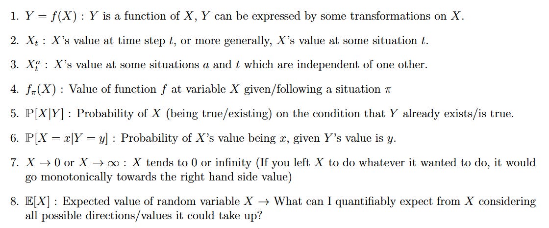
If only I had written this blog 6 months back, I could have moved on to write and blog about much more interesting stuff. But anyway, here we are - A gentle (hopefully intuitive) introduction to RL. Before we start, check out this primer on language and notation at the end of the doc - the best way to tackle difficult math, I have found, is to know how to speak math as it is written. This gets easier with time, but I’ll try to keep this primer resourceful at least for our purposes currently. I have tried to also add alt text over the formulas, so you can verify their verbalisation.

In this blog, I’d want to cover an intuitive understanding of RL and some of its bedrock ideas around environment, reward, state, Markov Processes, policy and value functions. A majority of the content is inspired and taken from 3 main sources - my notes from UCL and David Silver’s RL course, IITM and B. Ravindran’s RL course and the amazing Sutton and Barto Reinforcement Learning - An Introduction.

First Dip

Machine Learning is a paradigm under AI where given some historical data and expected outputs, a model is learned that could potentially derive outputs with new unseen data. It is nice because we have so much data that finding patterns and deriving a function through automation is fundamentally easier than ever. There are three kinds of machine learning methodologies, based on the existence of feedback or its timing along the training.

Supervised Learning - data and feedback are both instantly available.

Unsupervised Learning - data is available but feedback doesn’t exist.

Reinforcement Learning - data appears but the feedback is delayed.

Given ample literature on supervised and unsupervised learning and their applications, I’d jump straight to where we use RL.

RL is the study of sequential decision-making under uncertainty.

Here,

sequential - a paradigm that changes and modifies with time and interaction → much like the real world. I am not a ubiquitous narrator, but I (RL agent) actively participate in how I respond to the environment variables and how those variables change with my responses.

decision-making - I have the “agency” to choose a response (/action)

uncertainty - I don’t know what responses lead to what changes, initially and how good or bad they are because my feedback is delayed.

The basic RL Framework

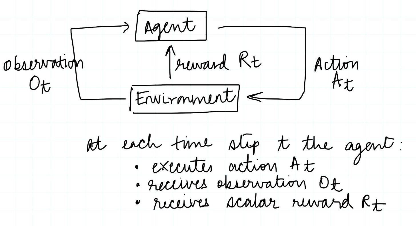
Terminology

• History: the sequence of observations, actions and rewards over the past. The history at time t denotes all the observable variables up to a time t. The future is dependent on this history.

\(H_t = A_1, O_1, R_1, A_2, …, A_t, O_t, R_t\)

• State: Summary of all the required information to determine what happens next. The state is a function of the history.

\(S_t = f(H_t)\)

• Environment State and Agent State:

  Environment State is the environment’s private representation - all the information that environment uses to pick the next observation/reward.

  Agent State is the agent’s internal representation - all the information the agent uses to pick the next action. And this is precisely all the information used by RL algorithms.

\(Environment State : S_t^e, Agent State : S_t^a\)

Components of an RL Agent

An RL agent may include one or more of these functional information -

• Policy function describes the agent’s behaviour

  • It is a map from state to action
  • A deterministic policy would mean that a unique action ensures the best reward whenever state S happens. A stochastic policy, on the other hand, does not guarantee this, and an action does not have a unique link to the state.

• Value function describes the utility or goodness of each state and/or action

  • The value function is a prediction of the future reward given the information state and available action choices. We want to choose the action that maximises the value function.

• Model function describes the agent’s representation of the environment.

  • A model predicts what the environment will do in response to a state and an action over that state.

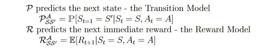
The majority of all RL algorithms are designed for optimising over these three components and making the agent better at maximising rewards.

The Markov Property

“The future is independent of the past given the present.”

This means that the state St is a sufficient statistic of the future. All of the history of observations, actions and rewards can be explained and encompassed through this one variable, and is sufficient to predict the next action and observation.

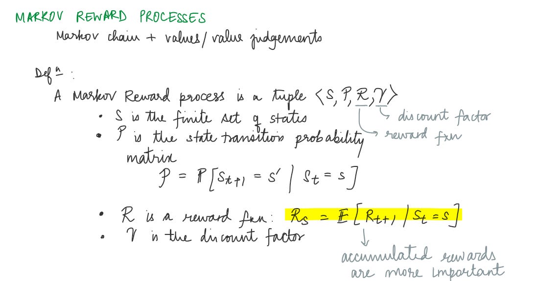
Markov Process: is a memoryless random process, i.e. a sequence of random states S1,S2,… with the Markov property. A Markov process (or Markov chain) is a tuple <S,P> where:

• S is a finite set of states

• P is a state-transition probability matrix

  • For a Markov state S and successor state S’, the state transition probability (PSS’)is the probability that given I am in state S and by taking some action, I go next to state S’. A state transition matrix P then defines these transition probabilities from all states S to all successor states S’.

\(P_{SS’} = P[S_{t+1} = s’|S_t=s]\)

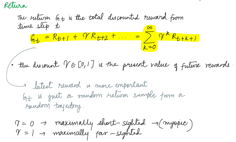
Why discount? To keep the math bounded and avoid infinite returns in cyclic markov chains. It is also more likely (wrt rich environments) that immediate rewards have more value in determining utility of an action than a delayed reward that’s harder to map. It is still possible to use discounted Markov reward processes if all sequences definitely terminate.

In the (hopefully soon) blogpost, I’d go deeper into the math of value functions, returns, the Bellman Equations and introduce the paradigm of dynamic programming in RL.

• The math and notation primer is here